The REMO model
Daniela Jacob
Max-Planck-Institut für Meteorologie, Hamburg
REMO was developed upon the request of the reviewers within the BMBF-Förderschwerpunkt Wasserkreislauf as the atmospheric component of the coupled atmosphere-hydrology model system. Development and application of this system was considered a central task within the international BALTEX (BALTIC Sea Experiment).
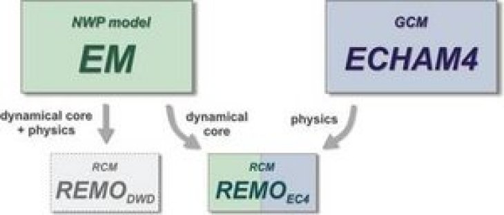
MPIfM (Max Planck Institute for Meteorology) was thus asked to develop the German BALTEX Model on the basis of the former numerical weather prediction model of the German Weather Service (EUROPA-MODELL, EM, Majewski 1991) in co-operation with DKRZ, DWD and GKSS. On 16 Nov 93 it was agreed between these parties to develop a regional model suitable for climate modelling and weather forecast which subsequently was named REMO. DWD and GKSS concentrated on modifications of the EM to use REMO in forecast mode (e.g. consecutive 30 hour forecasts without data assimilation) whilst DKRZ and MPIfM focussed on developments needed for the use of REMO in climate mode.
A version of the EM which allowed to carry out long term runs was modified at MPIfM to use surface pressure, horizontal wind components, temperature, water vapour and cloud water content as prognostic variables instead of surface pressure, horizontal wind components, total heat and total water content. The EM physical parameterisation scheme remained otherwise unchanged but the physical parameterisation scheme of the global climate model ECHAM4 (Roeckner et al. 1996) was implemented as an alternative option.
A major objective of BALTEX is to understand and quantify the water and energy cycles over the Baltic Sea and its drainage basin. Therefore the validation of REMO concentrated on the hydrological components of the water cycle. Simulation results of long runs up to ten years using ECMWF re-analysis data as lateral boundary conditions have been compared successfully with observations (Jacob 2001). Furthermore, REMO participated in a model inter-comparison during the PIDCAP period (Pilot study of Intense Data Collection and Analyses of Precipitation) involving eight regional models in total (Jacob et al. 2001).
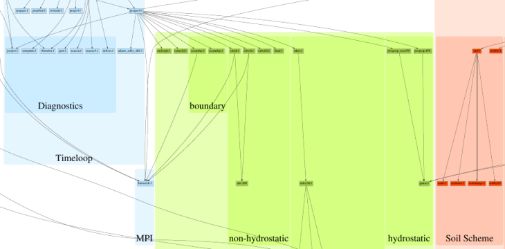
REMO runs on various platforms including scalar and vector computers such as CRAY, NEC, IBM, DEC, HP, SGI and Linux workstations. A parallel version (MPI) is also in use. Horizontal resolutions between 1/10° and 1° are currently used for simulations covering time ranges from days to centuries with both parameterisations. The following regions have been investigated with REMO: Europe, Arctic, Antarctic, Siberia, Indonesia, India, Brazil, Peru, Africa, North America, Baltic Sea, North Sea, North Atlantic, Pacific.
The atmospheric model REMO is coupled to three different hydrology models and three ocean/sea-ice models. An on-line chemistry module for tropospheric chemistry is available.
REMO is used by about 15 institutes in Germany, France, Switzerland, Greece and China. Interest in its use has been expressed by a number of further institutes in Germany and beyond. Numerous other institutes analyse the output generated by REMO.
During the next four years, REMO will be used as the atmospheric component of BALTIMOS (BALTEX Integral MOdel System) which is the BMBF funded nine partner consortium Development and validation of a coupled model system for the Baltic region. BALTIMOS consists of the modules: atmosphere, sea ice, ocean, land surface and hydrology. The main activity will be the validation of the fully coupled system. Furthermore, REMO is embedded in several other national and international projects for the next years.
Model Characteristics
References
- Jacob, D., U. Andrae, G. Elgered, C. Fortelius, L. P. Graham, S. D. Jackson, U. Karstens, Chr. Koepken, R. Lindau, R. Podzun, B. Rockel, F. Rubel, H.B. Sass, R.N.D. Smith, B.J.J.M. Van den Hurk, X. Yang, 2001: A Comprehensive Model Intercomparison Study Investigating the Water Budget during the BALTEX-PIDCAP Period. Meteorology and Atmospheric Physics, Vol.77, Issue 1-4, 19-43.
- Jacob, D., 2001: A note to the simulation of the annual and inter-annual variability of the water budget over the Baltic Sea drainage basin. Meteorology and Atmospheric Physics, Vol.77, Issue 1-4, 61-73.
- Majewski, D, 1991: The Europa-Modell of the Deutscher Wetterdienst. ECMWF Seminar on numerical methods in atmospheric models, Vol.2, 147-191.
- Roeckner, E., K. Arpe, L. Bengtsson, M. Christoph, M. Claussen, L. Dümenil, M. Esch, M. Giorgetta, U. Schlese, U. Schulzweida, 1996: The atmospheric general circulation model ECHAM-4: Model description and simulation of the present day climate. Max-Planck-Institut für Meteorologie Report No. 218.
REMO - Model Characteristics
REMO has two different parameterization schemes - the original one called DWD physics and additional the ECHAM4 physics, which is the same parameterization scheme as in the global climate model at MPI. The dynamical scheme is in both cases identical. REMO at MPI can be integrated in forecast as well as in climate mode.
Dynamical Scheme
- Rotated spherical grid
- Arakawa-C-grid
- Second order horizontal and vertical differences
- Leap-frog time stepping with semi-implicit correction and Asselin-filter
- Fourth-order linear horizontal diffusion of momentum, temperature and water content
- Hybrid vertical coordinates
- Prognostic variables: surface pressure, temperature, horizontal wind components, water vapour content, cloud water content.
- Lateral boundary formulation after Davies (1976), which adjusts the prognostic variables in a boundary zone of 8 grid boxes.
Physical parametrizations:
DWD physics
- Soil model with 2 layers for the heat budget and 3 layers for the water budget including a snow and interception storage (Jacobsen and Heise, 1982). Monthly mean climatological values are prescribed below these layers.
- Vertical diffusion after Louis (1979) for the Prandtl layer, extended level-2 scheme after Mellor and Yamada (1974) in the Ekman layer and the free atmosphere including modifications in the presence of clouds.
- Delta-two-stream radiation scheme after Ritter and Geleyn (1992) with 8 spectral intervals (3 solar, 5 thermal). The cloud radiative properties depend on the cloud water for saturated layers. In subsaturated layers a fractional cloud cover is diagnosed from the relative humidity and the cloud water content is set to 0.5 % of the saturation value. In the case of convective clouds the cloud cover is set to 0.2 and the cloud water content is set to 1 % of the saturation value. No parameterization of the radiative properties of ice clouds is included.
- Grid-scale cloud microphysics parameterization of the Kessler-type with water vapour and cloud water as a prognostic variables. Rainfall and snowfall rates are derived diagnostically assuming stationarity and neglecting advection.
- Mass-flux convection scheme after Tiedke (1989)
Modified ECHAM4 physics:
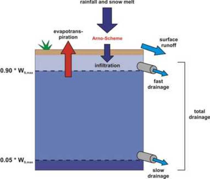
- Soil processes heat transfer: diffusion equation solver in a 5-layer model with zero heat flux at the bottom (10m); water budget equation for three reservoirs: soil moisture, interception reservoir (vegetation), snow; runoff scheme: based on catchment considerations including sub-grid scale variations of field capacity over inhomogeneous terrain (Dümenil and Todini, 1992)
- Vertical diffusion and surface fluxes: turbulent surface fluxes are calculated from Monin-Obukhov similarity theory (Louis, 1979) with a higher order closure scheme for the transfer coefficients of momentum, heat, moisture and cloud water within and above PBL. The eddy diffusion coefficients are calculated as functions of the turbulent kinetic energy E.
- Radiation after Morcrette et al. (1986) with modifications for additional greenhouse gases, 14.6 µm band of ozone and various types of aerosols. Continuum absorption after Giorgetta and Wild (1995).
- Stratiform clouds: water content is calculated from a budget equation including sources and sinks due to phase changes and precipitation formation by coalescense of cloud droplets and gravitational settling of ice crystals (Sundquist, 1978). The convective cloud water detrained at the top of cumulus clouds is used as a source term in stratiform cloud water equation (Roeckner et al., 1996)
- Cumulus convection: Mass flux convection scheme after Tiedtke (1989) with modifications after Nordeng (1994)
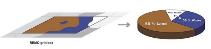
- fractional surface cover: land, water, sea ice (Semmler, 2002)
- freezing and thawing of soil water (Semmler, 2002)
- monthly variation of vegetation parameters: background albedo, leaf area index, vegetation ratio (Rechid & Jacob, 2006)
- snow-free land surface albedo as a function of vegetation phenology based on MODIS data (Rechid et al, 2009)
References
- Davies, H.C., 1976: A lateral boundary formulation for multi-level prediction models. Quart. J. R. Meteor. Soc., 102, 405-418.
- Deutsches Klima Rechenzentrum (DKRZ), 1992: The ECHAM3 general circulation model. DKRZ Technical Report, No. 6, edited by Modellbetreuungsgruppe, Hamburg.
- Dümenil, L. and E. Todini, 1992: A rainfall-runoff scheme for use in the Hamburg climate model . In: Advances in Theoretical Hydrology, A Tribute to James Dooge (Ed. J.P. O'Kane). European Geophysical Society Series on Hydrological Sciences, 1, Elsevier Press Amsterdam, 129-157
- Giorgetta, M. and M. Wild, 1995: The water vapour continuum and its representation in ECHAM4. Max-Planck Institut für Meteorologie Report No. 162, 38pp.
- Jacobsen, I. and E. Heise, 1982: A new economic method for the computation of the surface temperature in numerical models. Beitr. Phys. Atm., 55, 128-141.
- Louis, J.-F., 1979: A parametric model of vertical eddy fluxes in the atmosphere. Boundary-Layer Meteor., 17, 187-202.
- Mellor, G.L. and T. Yamada, 1974: A hierarchy of turbulence closure models for planetary boundary layers. J. Atmos. Sci., 31, 1791-1806.
- Morcrette, j.-j., L. Smith and Y. Fourquart, 1986: Pressure and temperature dependance of the absorption in longwave radiation parameterizations. Beitr. Phys. Atmos. 59, 455-469.
- Nordeng, T.E., 1994: Extended versions of the convective parametrization scheme at ECMWF and their impact on the mean and transient activity of the model in the tropics. ECMWF Research Department, Technical Momorandum No. 206, October 1994, 41 pp, European Centre for Medium Range Weather Forecasts, Reading, UK.
- Rechid D., T.J. Raddatz and D. Jacob, 2009: Parameterization of snow-free land surface albedo as a function of vegetation phenology based on MODIS data and applied in climate modelling. Theor. Appl. Climatol., 95, 245–255
- Ritter, B. and J.-F. Geleyn, 1992: A comprehensive radiation scheme for numerical weather prediction models with potential applications in climate simulations. Mon. Wea. Rev., 120, 303-325.
- Roeckner, E., K. Arpe, L. Bentsson, M. Christoph, M. Claussen, L. Dümenil, M. Esch, M. Giorgetta, U. Schlese and U. Schulzweida, 1996: The atmospheric genaral circulation model ECHAM-4: Model description and simulation of present day climate. Max-Planck Institut für Meteorologie Report No. 218, 90 pp.
- Sundquist, H., 1978: A parameterization scheme for non-convective condensation including precipitation including prediction of cloud water content. Quart. J. R. Met. Soc., 104, 677-690.
- Tiedtke, M., 1989: A comprehensive mass flux scheme for cumulus parameterization in large scale models. Mon. Wea. Rev., 117, 1779-1800.